Using turtleFSI

Execute a run

turtleFSI is aimed to be user friendly, where all parameters can be controlled from the command line. We here provide an example on how to create your own problem file. First a quick recap on how to execute turtleFSI.

To run turtleFSI with all the default parameters you can execute:

turtleFSI

which will execute the default problem file turtle_demo.py with all the default parameter. In the folder where you executed the command there will be a folder turtle_demo_results/1 where you can find Visualization files, and under Checkpoint you can find a list of all parameters used in default_variables.pickle.

Note

The default number of time steps is set to 30, which takes a couple of minutes to execute on a normal desktop. To re-create the video shown in readme set the end time (T) to 15 seconds. This will take some time to run, but you can look at the intermediate results in turtle_demo_results/1 in paraview while running the simulation.

To run a specific problem file, run:

turtleFSI --problem [path_to_problem]

To get an overview of all parameters, please run:

turtleFSI -h

Built-in functionality

TurtleFSI is designed to be lightweight and generic, but we have added to features generally of interest: checkpointing/restart, and storing files for visualization.

For checkpointing you can set the variable --checkpoint-step to set the checkpoint frequency, i.e., how often a checkpoint should be stored. To restart from a previous checkpoint, use the command --restart-folder [folder]/[sub-folder]. Note that the variables from the previous simulation will overwrite any parameters defined in set_problem_parameters or on the commandline. If you need to change a parameter from the previous checkpoint file (for instance, end time T), you can still do it by explicitly redefining the variable in the initiate function.

To set how often you save files for visualization you can set --save-step. Note that the default is 10.

Setting parameters

All the default parameters are set in the problem/__init__.py file. Problem specific parameters are then overwritten in the problem file under set_problem_parameters or from the command line. In summary; the parameters will be updated in the following order: default parameters < set_problem_parameters < command line (< checkpointing) < other problem specific functions.

Create your own problem file

We have created a step-by-step explanation, see the below, on how you can create your own problem file.

For all numerical problems we have to specify a set parameters, provide a mesh and boundary conditions, how to solve the equations, and finally specify which metric we are interested in measuring. In turtleFSI problem file you can define up to seven functions which provides the solver with the above mentioned information. Listed in the order they are first executed:

• set_problem_parameters
• get_mesh_domain_and_boundaries
• initiate (optional)
• create_bcs
• pre_solve (optional)
• post_solve (optional)
• finished (optional)

set_problem_parameters

This function is for defining parameters of the problem like: time step size dt, end time T, and physical parameters of the problem. To see a full list of the default parameters, we refer to the default_variables defined in turtleFSI/problems/__init__.py. Please note that you can, and should, also define other problem specific variables in default_variables, for instance, geometry information like hight and length of the problem is of interest to the problem you are solving.

In the set_problem_parameters function, you have the possibility to set your problem parameters within the default_variables dictionary. However, keep in mind that any command line arguments will overwrite the default_variables.

A simple example of this function can look like this:

def set_problem_parameters(default_variables, **namespace):
    # Overwrite default values
    default_variables.update(dict(
        T=15,                          # End time [s]
        dt=0.005,                      # Time step [s]
        theta=0.505,                   # theta value (0.5 + dt), shifted Crank-Nicolson scheme
        Um=1.0,                        # Max. velocity inlet [m/s]
        rho_f=1.0E3,                   # Fluid density [kg/m3]
        mu_f=1.0,                      # Fluid dynamic viscosity [Pa.s]
        rho_s=1.0E3,                   # Solid density [kg/m3]
        mu_s=5.0E4,                    # Solid shear modulus or 2nd Lame Coef. [Pa]
        lambda_s=4.5E5,                # Solid 1st Lame Coef. [Pa]
        nu_s=0.45,                     # Solid Poisson ratio [-]
        dx_f_id=1,                     # ID of marker in the fluid domain
        dx_s_id=2,                     # ID of marker in the solid domain
        extrapolation="biharmonic",    # laplace, elastic, biharmonic, no-extrapolation
        extrapolation_sub_type="constrained_disp",  # ["constant", "small_constant", "volume", "volume_change", "constrained_disp", "constrained_disp_vel"]
        recompute=15,                  # recompute the Jacobian matrix every "recompute" Newton iterations
        folder="turtle_demo_results"), # name of the folder to save the data
        save_step=1                    # frequency of data saving
     )
     return default_variables

Note

The parameter extrapolation here refers to mesh lifting operator, i.e., how to de extrapolate the deformation of the solid into the fluid to create an ALE frame of reference. Laplace is the cheapest in terms of computational cost, but is less robust for large deformations and sharp edges. In contrast, biharmonic is very robust, but at the cost of computational efficiency and increased memory load.

get_mesh_domain_and_boundaries

The function is essential and unique for every problem, and has to be provided for the problem file to run. Here you read or define your mesh, domain markers, and boundary markers. In turtle_demo.py we read the mesh data from pre-existing “.xdmf” mesh files. In contrast to defining the domain and boundary markers using FEniCS functions, like in the the ‘Turek flag’-example (TF_fsi.py).

pygmsh and meshio are relevant tools to create geometries. For any question regarding meshing, we refer to the FEniCS documentation and discourse group.

In turtle_demo.py, the function looks like this:

def get_mesh_domain_and_boundaries(args, **namespace):
    mesh_folder = path.join(path.dirname(path.abspath(__file__)), "..", "mesh", "turtle_demo")

    # In this example, the mesh and markers are stored in the 3 following files
    mesh_path = path.join(mesh_folder, "turtle_mesh.xdmf")     # mesh geometry
    domains_marker_path = path.join(mesh_folder, "mc.xdmf")    # marker over the elements (domains)
    boundaries_marker_path = path.join(mesh_folder, "mf.xdmf") # markers of the segments (boundaries)

    # "mesh" collects the mesh geometry of the entire domain (fluid + solid).
    # In this example, we import a mesh stored in a .xdmf file, but other formats
    # are supported such as .xml files.
    mesh = Mesh()
    xdmf = XDMFFile(MPI.comm_world, mesh_path)
    xdmf.read(mesh)

    # "domains" collects the element markers of the fluid domain (marked as 1)
    # and the solid domain (marked as 2).
    domains = MeshFunction("size_t", mesh, mesh.geometry().dim())
    xdmf = XDMFFile(MPI.comm_world, domains_marker_path)
    xdmf.read(domains)

    # "boundaries" collects the boundary markers that are used to apply the
    # Dirichlet boundary conditions on both the fluid and solid domains.
    # Marker values ranging from 11 to 15.
    mesh_collection = MeshValueCollection("size_t", mesh, mesh.geometry().dim() - 1)
    xdmf = XDMFFile(MPI.comm_world, boundaries_marker_path)
    xdmf.read(mesh_collection)
    boundaries = cpp.mesh.MeshFunctionSizet(mesh, mesh_collection)

    return mesh, domains, boundaries

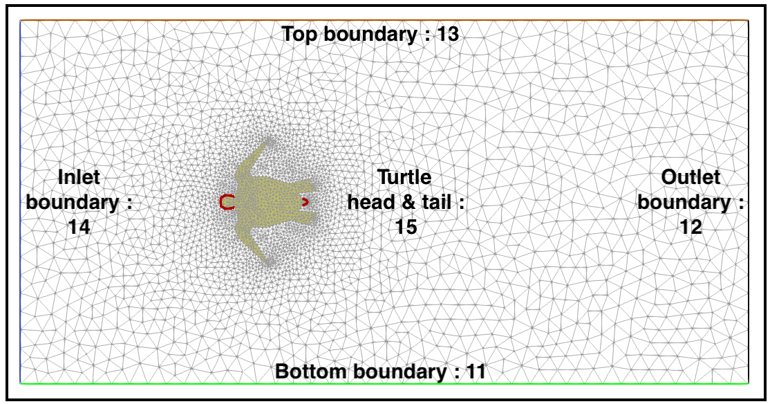
Domain boundaries.

initiate

This function is not strictly necessary, but can be used to initiate variables before entering the time loop of the simulation. Here we have no need for that, and have therefore not included it. See TF_fsi.py for an example.

create_bcs

The function create_bcs is used to define the boundary conditions of the problem to be solved, and is required for the problem file to run. In turtle_demo.py, the inlet boundary condition is defined the Inlet class, which inherits the FEniCS UserExpression class. This class is then used in the function create_bcs to prescribe Dirichlet boundary condition to the inlet velocity. When defining the boundary conditions to specific domain regions or boundaries, make sure to be consistent with the markers provided in get_mesh_domain_and_boundaries:

class Inlet(UserExpression):
    def __init__(self, Um, **kwargs):
        self.t = 0.0
        self.t_ramp = 0.5  # time to ramp-up to max inlet velocity (from 0 to Um)
        self.Um = Um       # Max. velocity inlet [m/s]
        super().__init__(**kwargs)

    def update(self, t):
        self.t = t
        if self.t < self.t_ramp:
            self.value = self.Um * np.abs(np.cos(self.t/self.t_ramp*np.pi)-1)/2  # ramp-up the inlet velocity
            print(self.value)
        else:
            Um_min = self.Um/6  # lower velocity during oscillations
            self.value = (self.Um-Um_min) * np.abs(np.cos(self.t/self.t_ramp*np.pi)-1)/2 + Um_min
            print(self.value)

    def eval(self, value, x):
        value[0] = self.value
        value[1] = 0

    def value_shape(self):
        return (2,)


def create_bcs(DVP, boundaries, Um, v_deg, extrapolation_sub_type, **namespace):
    if MPI.rank(MPI.comm_world) == 0:
        print("Create bcs")

    inlet = Inlet(Um, degree=v_deg)
    noslip = ((0.0, 0.0))

    # Segments indices (make sure of the consistency with the boundary file)
    bottom_id = 11  # segments at the bottom of the model
    outlet_id = 12  # segments at the outlet (right wall) of the model
    top_id = 13     # segments at the top (right wall) of the model
    inlet_id = 14   # segments at the inlet (left wall) of the model
    turtle_head_tail_id = 15   # segments along the head and tail of the turtle

    # Fluid velocity boundary conditions
    u_inlet = DirichletBC(DVP.sub(1), inlet, boundaries, inlet_id)
    u_bot = DirichletBC(DVP.sub(1).sub(1), (0.0), boundaries, bottom_id)  # slip in x-direction
    u_top = DirichletBC(DVP.sub(1).sub(1), (0.0), boundaries, top_id)     # slip in x-direction
    u_head_tail = DirichletBC(DVP.sub(1), noslip, boundaries, turtle_head_tail_id)

    # Pressure boundary conditions
    p_outlet = DirichletBC(DVP.sub(2), (0.0), boundaries, outlet_id)

    # List boundary conditions for the fluid
    bcs = [u_bot, u_top, u_inlet, p_outlet, u_head_tail]

    # Mesh uplifting boundary conditions
    d_inlet = DirichletBC(DVP.sub(0), noslip, boundaries, inlet_id)
    d_bot = DirichletBC(DVP.sub(0), noslip, boundaries, bottom_id)
    d_top = DirichletBC(DVP.sub(0), noslip, boundaries, top_id)
    d_outlet = DirichletBC(DVP.sub(0), noslip, boundaries, outlet_id)
    d_head_tail = DirichletBC(DVP.sub(0), noslip, boundaries, turtle_head_tail_id)

    # Add boundary conditions for the structure
    bcs += [d_bot, d_top, d_outlet, d_inlet, d_head_tail]:

    return dict(bcs=bcs, inlet=inlet)

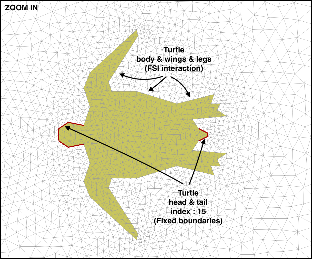
Boundaries between the fluid and structures and fixed boundaries.

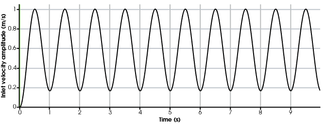
Inlet velocity amplitude variation with time as defined by the class Inlet().

pre_solve

This function is called within the time loop of the simulation before calling the solver at the given time step. In turtle_demo.py, we used this function to update the time variable of the Inlet expression used for the inlet boundary conditions:

def pre_solve(t, inlet, **namespace):
    # Update the time variable used for the inlet boundary condition
    inlet.update(t)

post_solve

This function is called within the time loop of the simulation after calling the solver at the given time step. In turtle_demo.py, we do not have any use for this function, but see TF_fsi.py for an example.

finished

Function called once at the end of the time loop. An example of use is given in the TF_fsi.py where text file are saved to store informations from the simulation:

def finished(folder, dis_x, dis_y, Drag_list, Lift_list, Time_list, **namespace):
    if MPI.rank(MPI.comm_world) == 0:
        np.savetxt(path.join(folder, 'Lift.txt'), Lift_list, delimiter=',')
        np.savetxt(path.join(folder, 'Drag.txt'), Drag_list, delimiter=',')
        np.savetxt(path.join(folder, 'Time.txt'), Time_list, delimiter=',')
        np.savetxt(path.join(folder, 'dis_x.txt'), dis_x, delimiter=',')
        np.savetxt(path.join(folder, 'dis_y.txt'), dis_y, delimiter=',')

Visualizing the result

Given that the parameter --save-step not was set larger than the number of time steps, there will be a folder: [folder]/[sub-folder]/Visualization with xdmf files that can be opened in a visualization probrem, for instance ParaView. Below we have visualized the pressure and velocity at 2.5 s.

Note

In order to visualize the deformation of the mesh in ParaView, you need to apply a Warp by Vector filter to the displacement.xdmf. You can control the scale of the deofrmation by adjusting the Scale Factor.

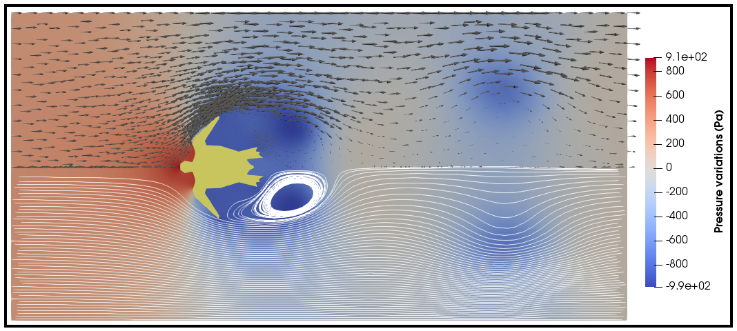
Pressure and velocity fields at 2.5 s. obtained by running the turtle_demo.py problem file.